A Christmas Present in Clojure
It’s time again for the annual State of Clojure Survey. I fill it out every year. And I love to read the responses. Please give the survey 15 minutes and become a statistic. This is one important way we, as a community, understand ourselves. Please fill it out by the end of the year.
I follow a number of people’s work, and one of them is Conal Elliott. I like that he’s very deliberate with his use of words. It makes me think a little harder. At some point, I heard him say that he didn’t think declarative was the right word. People tend to toss the word around and explain it as “saying what you want, not how to get it.” It’s the opposite of imperative, where you say how to get it. But Elliot is right. It’s not the word we want.
Like many problematic words, people use it in different senses. But the worst offense is that it’s not objective. It’s vibes. It’s relative. I’ve heard people say that map is declarative while a for loop is imperative. “With map, I just say what I want. But with a for loop, I have to say how to build the resulting array.” That may be true, but a for loop is very declarative relative to an if statement and a goto. Look at the anatomy of a for loop. You specify four things:
Initialization
Loop condition
Loop progress
Body of loop
And it magically executes the body of the loop until the loop condition is met. How does it do it? You never specified how. Which means it’s declarative. And I’ve implemented map many times over the years. I know how it’s working its wizardry. Which means it’s imperative.
These words just are not what we’re looking for. The main problem I have with the term declarative as we use it is that it’s all about ignorance. People say SQL is declarative because they don’t know how the query engine works. Once you learn how it works, you begin to write SQL to control how it runs.
Elliot suggests we instead use the term denotational, borrowed from the practice of Denotational Semantics. Denotational Semantics is a method for formally specifying the semantics of a programming language or construct in terms of lambda calculus. It contrasts with Operational Semantics, which is more like how a compiler might translate a language to machine code. If you squint, we want to replace declarative with denotational and replace imperative with operational.
In denotational programming, we specify how to derive the meaning of one expression by combining the meanings of the subexpressions. Even if we know what’s happening under the hood, the derivation of meaning is clear. Reasoning can be done locally. In operational semantics, we may get a good idea of how a feature can be implemented in assembly, but we have trouble simulating it in our head because of the many possible states the machine can be in. It is much harder to formalize and prove properties about it.
When we’re doing good functional programming, it’s much more on the denotational side. We’re defining one function in terms of other functions. We’re embedded in a lambda calculus, so it’s very comfortable to do.
I think there’s another correspondence, which is between operational/denotational and implementation/specification. I think one of the important skills that differentiates of senior from a junior engineer is the ability to separate implementation from specification. A junior is just trying to get something working. But a senior engineer thinks about the meanings they want to represent apart from how to represent them.
This brings me to the working title of my book, Runnable Specifications. The idea is one I borrowed from Alan Kay. He says the ultimate goal for a programming system is to be able to run the specification, not translate it into an implementation. You want to write down a question and run it to get the answer. He’s talking about a denotational way of programming where you write programs directly in the language of the domain.
Denotational differs from declarative in one other way. Denotational programming deals with how meanings are combined to form new meanings. Declarative can but often does not deal with combining meanings. I look at SQL again as an example of something that doesn’t make composition easy.
Well, I don’t think I really destroyed the term declarative as much I imagined I would at the beginning of this essay. That’s okay. I think denotational is a strong enough replacement that it doesn’t really need to be destroyed. The biggest downside to the word is that people don’t know what it means. But I do!

Translations: Russian
Syntax highlighting is a tool. It can help you read code faster. Find things quicker. Orient yourself in a large file.
Like any tool, it can be used correctly or incorrectly. Let’s see how to use syntax highlighting to help you work.
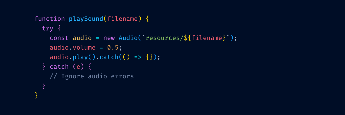
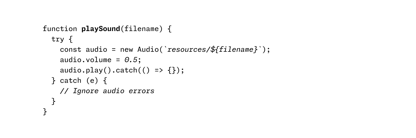
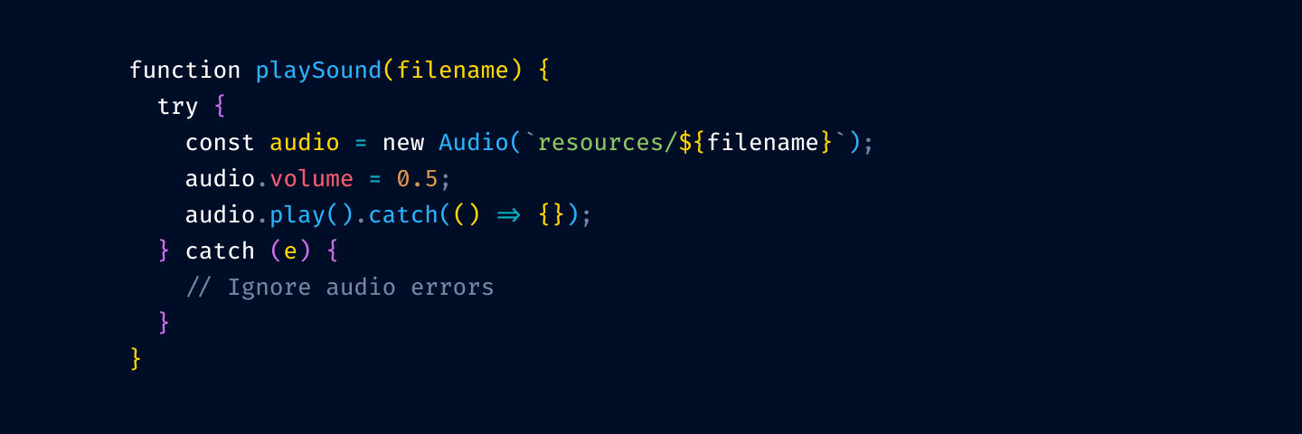
Most color themes have a unique bright color for literally everything: one for variables, another for language keywords, constants, punctuation, functions, classes, calls, comments, etc.
Sometimes it gets so bad one can’t see the base text color: everything is highlighted. What’s the base text color here?
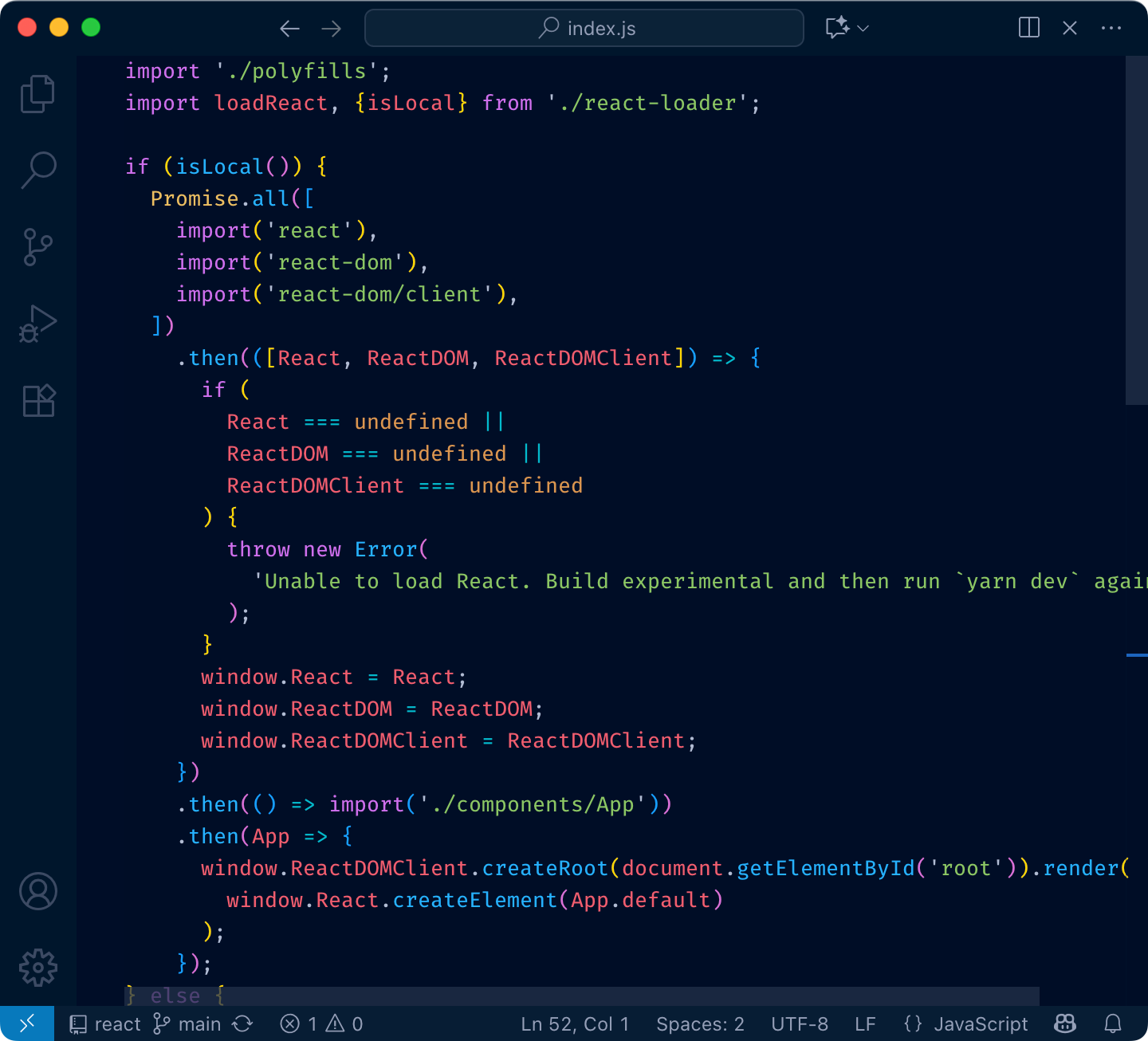
The problem with that is, if everything is highlighted, nothing stands out. Your eye adapts and considers it a new norm: everything is bright and shiny, and instead of getting separated, it all blends together.
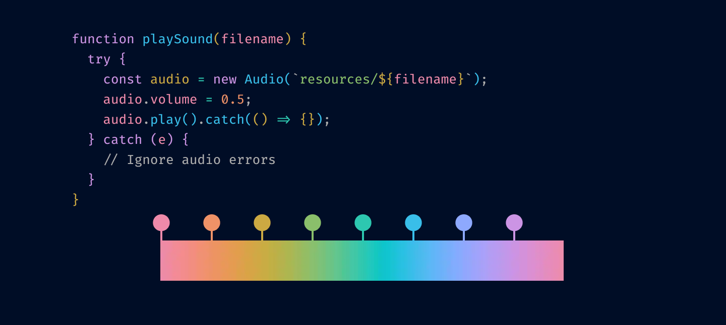
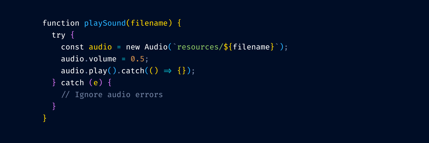
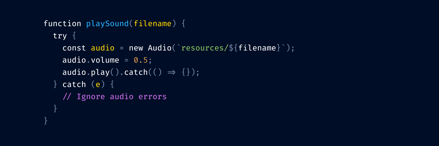
Here’s a quick test. Try to find the function definition here:
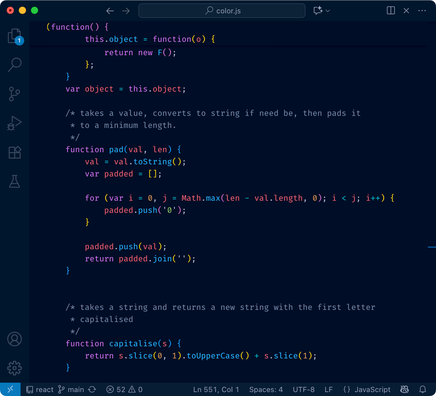
and here:
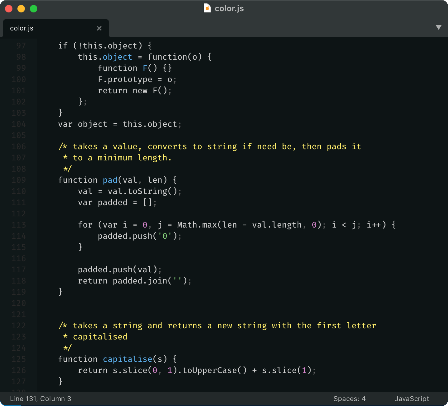
See what I mean?
So yeah, unfortunately, you can’t just highlight everything. You have to make decisions: what is more important, what is less. What should stand out, what shouldn’t.
Highlighting everything is like assigning “top priority” to every task in Linear. It only works if most of the tasks have lesser priorities.
If everything is highlighted, nothing is highlighted.
There are two main use-cases you want your color theme to address:
1 is a direct index lookup: color → type of thing.
2 is a reverse lookup: type of thing → color.
Truth is, most people don’t do these lookups at all. They might think they do, but in reality, they don’t.
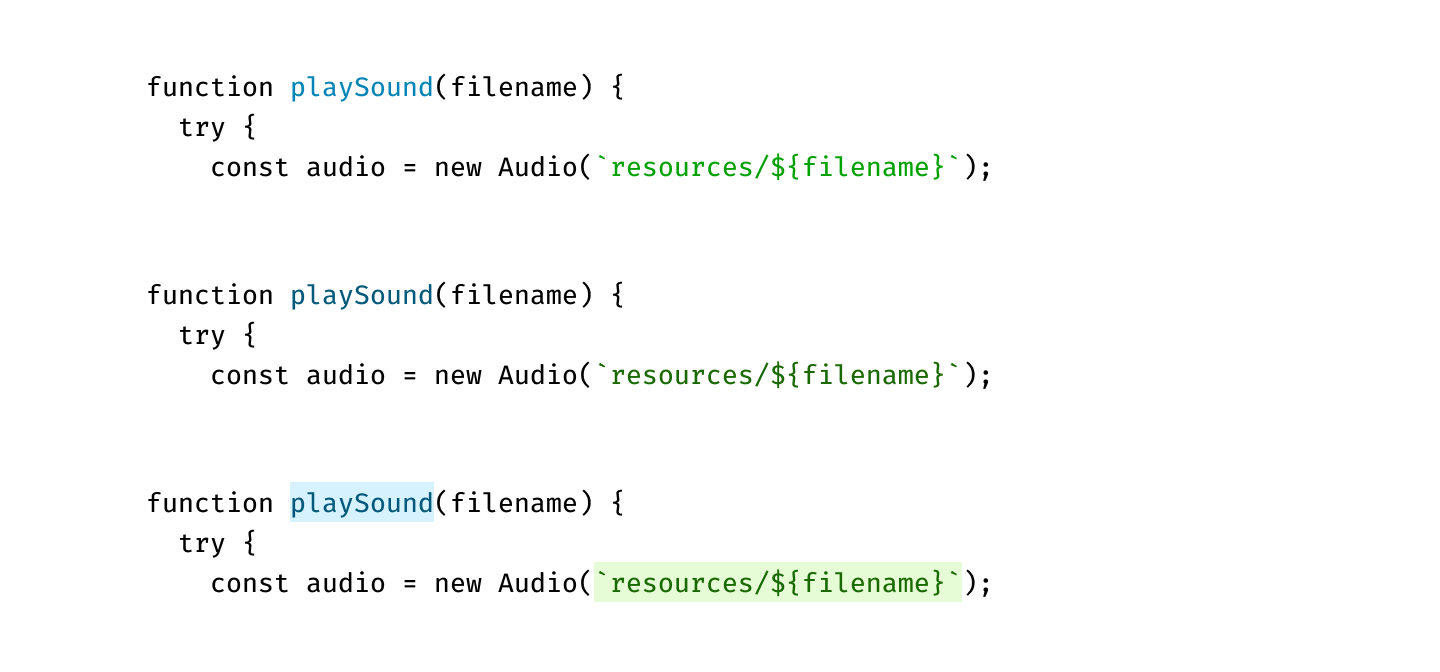
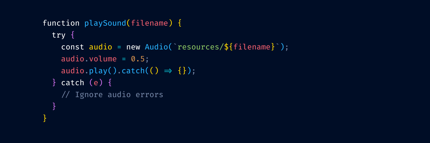
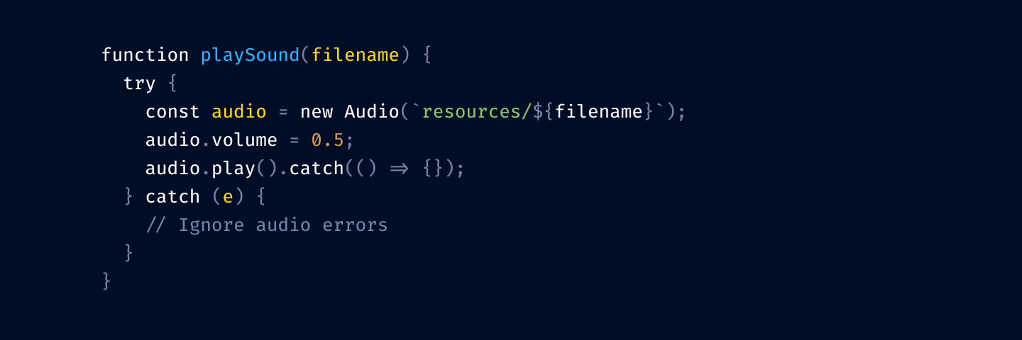
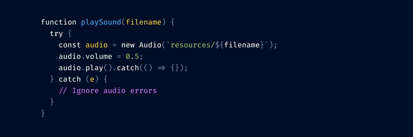
Let me illustrate. Before:
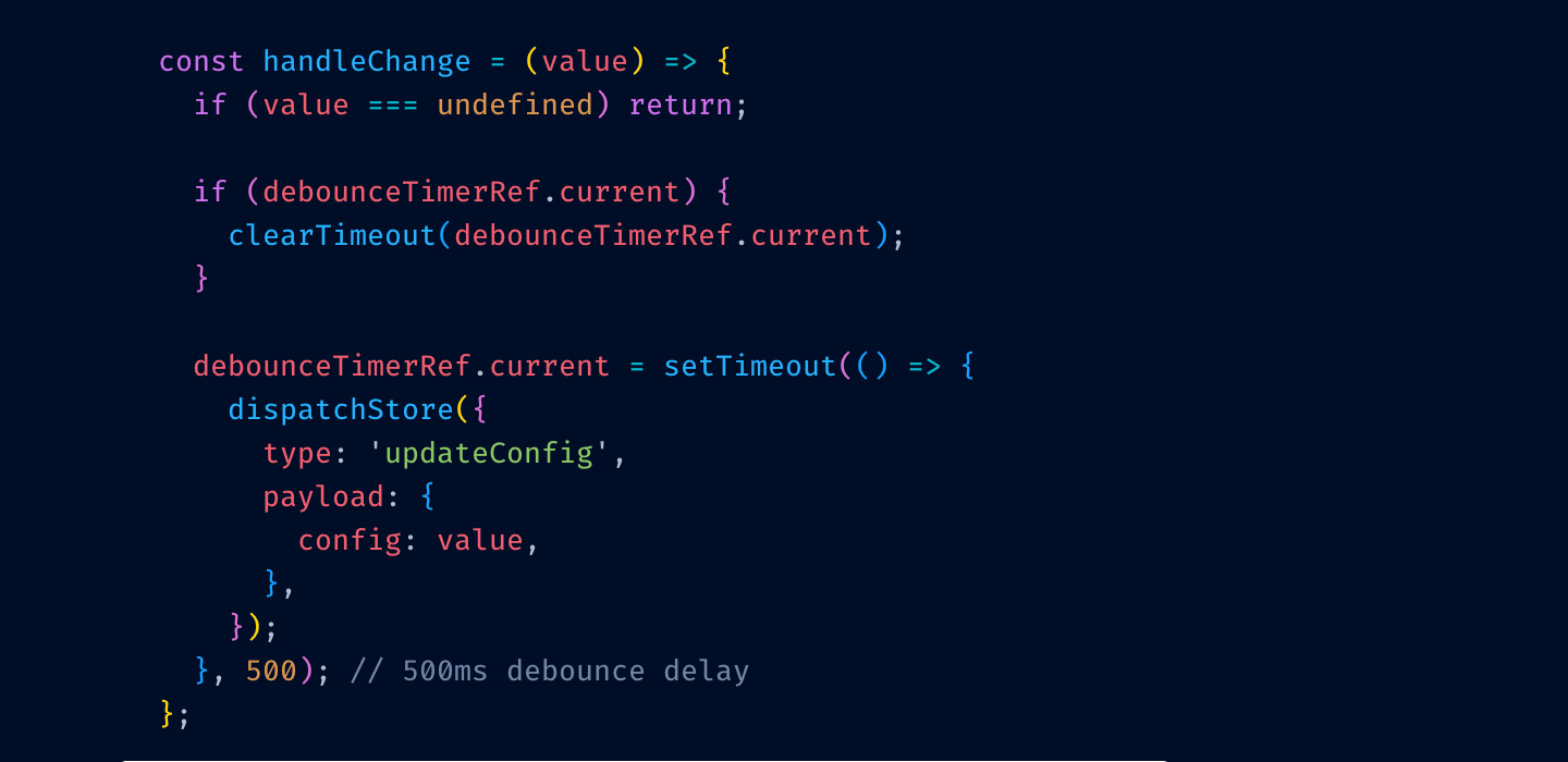
After:
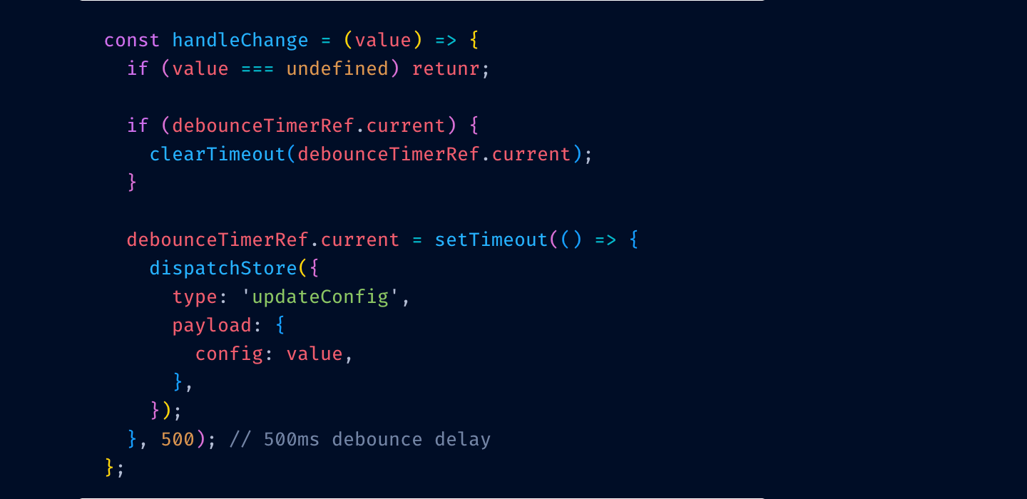
Can you see it? I misspelled return for retunr and its color switched from red to purple.
I can’t.
Here’s another test. Close your eyes (not yet! Finish this sentence first) and try to remember what color your color theme uses for class names?
Can you?
If the answer for both questions is “no”, then your color theme is not functional. It might give you comfort (as in—I feel safe. If it’s highlighted, it’s probably code) but you can’t use it as a tool. It doesn’t help you.
What’s the solution? Have an absolute minimum of colors. So little that they all fit in your head at once. For example, my color theme, Alabaster, only uses four:
That’s it! And I was able to type it all from memory, too. This minimalism allows me to actually do lookups: if I’m looking for a string, I know it will be green. If I’m looking at something yellow, I know it’s a comment.
Limit the number of different colors to what you can remember.
If you swap green and purple in my editor, it’ll be a catastrophe. If somebody swapped colors in yours, would you even notice?
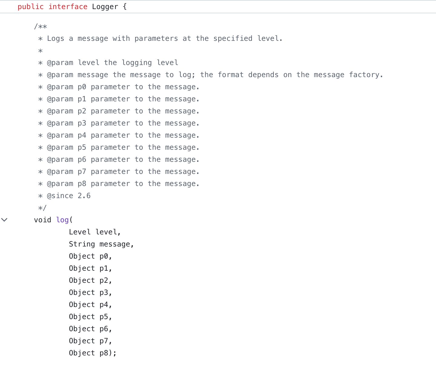
Something there isn’t a lot of. Remember—we want highlights to stand out. That’s why I don’t highlight variables or function calls—they are everywhere, your code is probably 75% variable names and function calls.
I do highlight constants (numbers, strings). These are usually used more sparingly and often are reference points—a lot of logic paths start from constants.
Top-level definitions are another good idea. They give you an idea of a structure quickly.
Punctuation: it helps to separate names from syntax a little bit, and you care about names first, especially when quickly scanning code.
Please, please don’t highlight language keywords. class, function, if, elsestuff like this. You rarely look for them: “where’s that if” is a valid question, but you will be looking not at the if the keyword, but at the condition after it. The condition is the important, distinguishing part. The keyword is not.
Highlight names and constants. Grey out punctuation. Don’t highlight language keywords.
The tradition of using grey for comments comes from the times when people were paid by line. If you have something like
of course you would want to grey it out! This is bullshit text that doesn’t add anything and was written to be ignored.
But for good comments, the situation is opposite. Good comments ADD to the code. They explain something that couldn’t be expressed directly. They are important.
So here’s another controversial idea:
Comments should be highlighted, not hidden away.
Use bold colors, draw attention to them. Don’t shy away. If somebody took the time to tell you something, then you want to read it.
Another secret nobody is talking about is that there are two types of comments:
Most languages don’t distinguish between those, so there’s not much you can do syntax-wise. Sometimes there’s a convention (e.g. -- vs /* */ in SQL), then use it!
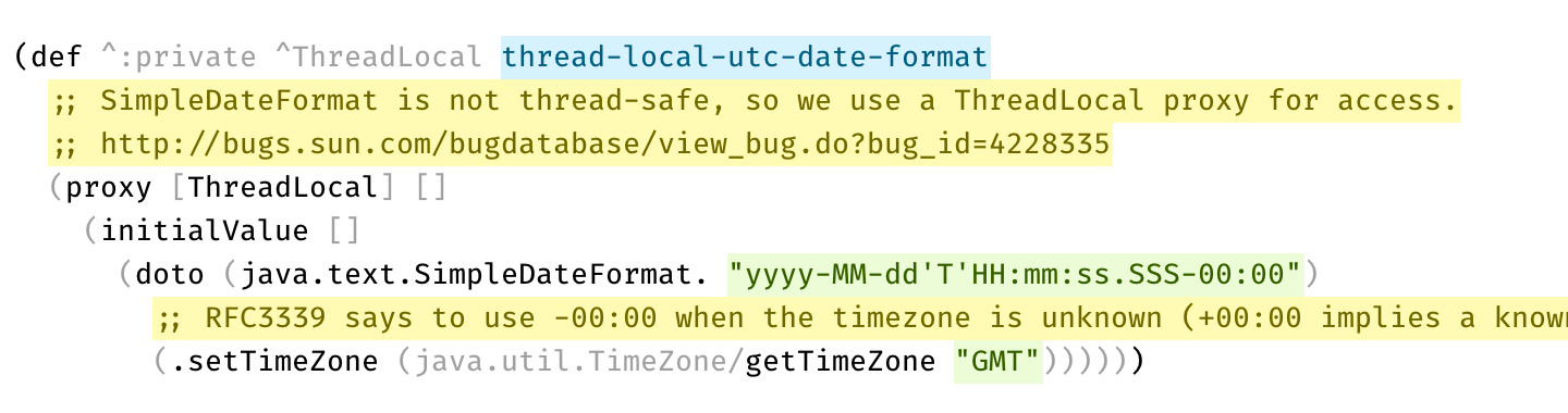
Here’s a real example from Clojure codebase that makes perfect use of two types of comments:
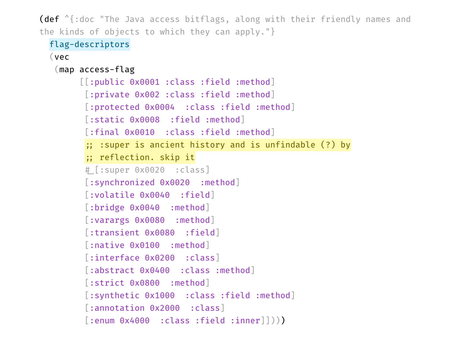 Disabled code is gray, explanation is bright yellow
Per statistics, 70% of developers prefer dark themes. Being in the other 30%, that question always puzzled me. Why?
And I think I have an answer. Here’s a typical dark theme:
and here’s a light one:
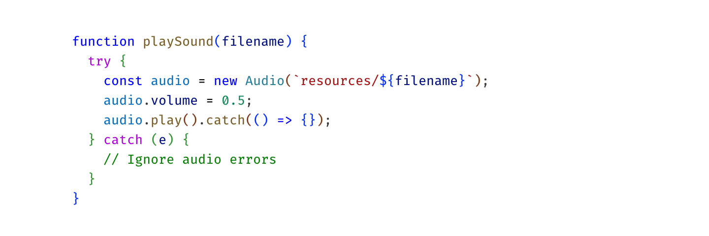
On the latter one, colors are way less vibrant. Here, I picked them out for you:
 Notice how many colors there are. No one can remember that many.
This is because dark colors are in general less distinguishable and more muddy. Look at Hue scale as we move brightness down:
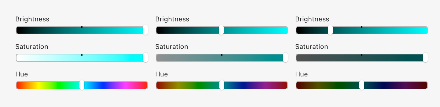
Basically, in the dark part of the spectrum, you just get fewer colors to play with. There’s no “dark yellow” or good-looking “dark teal”.
Nothing can be done here. There are no magic colors hiding somewhere that have both good contrast on a white background and look good at the same time. By choosing a light theme, you are dooming yourself to a very limited, bad-looking, barely distinguishable set of dark colors.
So it makes sense. Dark themes do look better. Or rather: light ones can’t look good. Science ¯\_(ツ)_/¯
But!
But.
There is one trick you can do, that I don’t see a lot of. Use background colors! Compare:
The first one has nice colors, but the contrast is too low: letters become hard to read.
The second one has good contrast, but you can barely see colors.
The last one has both: high contrast and clean, vibrant colors. Lighter colors are readable even on a white background since they fill a lot more area. Text is the same brightness as in the second example, yet it gives the impression of clearer color. It’s all upside, really.
UI designers know about this trick for a while, but I rarely see it applied in code editors:
If your editor supports choosing background color, give it a try. It might open light themes for you.
Don’t use. This goes into the same category as too many colors. It’s just another way to highlight something, and you don’t need too many, because you can’t highlight everything.
In theory, you might try to replace colors with typography. Would that work? I don’t know. I haven’t seen any examples.
 Using italics and bold instead of colors
Some themes pay too much attention to be scientifically uniform. Like, all colors have the same exact lightness, and hues are distributed evenly on a circle.
This could be nice (to know if you have OCD), but in practice, it doesn’t work as well as it sounds:
 OkLab l=0.7473 c=0.1253 h=0, 45, 90, 135, 180, 225, 270, 315
The idea of highlighting is to make things stand out. If you make all colors the same lightness and chroma, they will look very similar to each other, and it’ll be hard to tell them apart.
Our eyes are way more sensitive to differences in lightness than in color, and we should use it, not try to negate it.
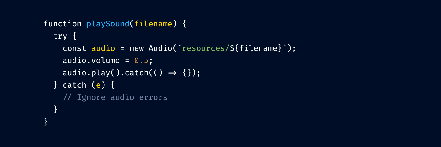
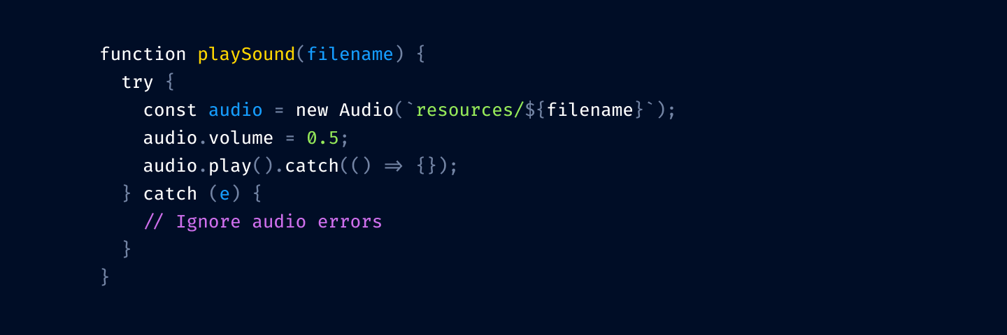
Let’s apply these principles step by step and see where it leads us. We start with the theme from the start of this post:
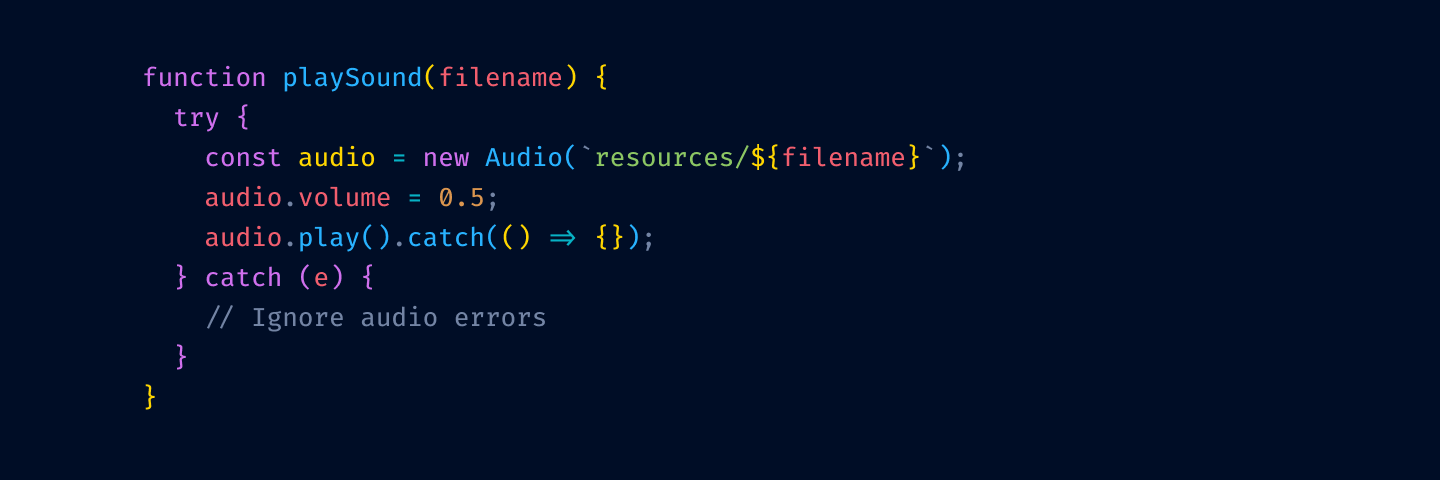
First, let’s remove highlighting from language keywords and re-introduce base text color:
Next, we remove color from variable usage:
and from function/method invocation:
The thinking is that your code is mostly references to variables and method invocation. If we highlight those, we’ll have to highlight more than 75% of your code.
Notice that we’ve kept variable declarations. These are not as ubiquitous and help you quickly answer a common question: where does thing thing come from?
Next, let’s tone down punctuation:
I prefer to dim it a little bit because it helps names stand out more. Names alone can give you the general idea of what’s going on, and the exact configuration of brackets is rarely equally important.
But you might roll with base color punctuation, too:
Okay, getting close. Let’s highlight comments:
We don’t use red here because you usually need it for squiggly lines and errors.
This is still one color too many, so I unify numbers and strings to both use green:
Finally, let’s rotate colors a bit. We want to respect nesting logic, so function declarations should be brighter (yellow) than variable declarations (blue).
Compare with what we started:
In my opinion, we got a much more workable color theme: it’s easier on the eyes and helps you find stuff faster.
I’ve been applying these principles for about 8 years now.
I call this theme Alabaster and I’ve built it a couple of times for the editors I used:
It’s also been ported to many other editors and terminals; the most complete list is probably here. If your editor is not on the list, try searching for it by name—it might be built-in already! I always wondered where these color themes come from, and now I became an author of one (and I still don’t know).
Feel free to use Alabaster as is or build your own theme using the principles outlined in the article—either is fine by me.
As for the principles themselves, they worked out fantastically for me. I’ve never wanted to go back, and just one look at any “traditional” color theme gives me a scare now.
I suspect that the only reason we don’t see more restrained color themes is that people never really thought about it. Well, this is your wake-up call. I hope this will inspire people to use color more deliberately and to change the default way we build and use color themes.
I have a weird relationship with statistics: on one hand, I try not to look at it too often. Maybe once or twice a year. It’s because analytics is not actionable: what difference does it make if a thousand people saw my article or ten thousand?
I mean, sure, you might try to guess people’s tastes and only write about what’s popular, but that will destroy your soul pretty quickly.
On the other hand, I feel nervous when something is not accounted for, recorded, or saved for future reference. I might not need it now, but what if ten years later I change my mind?
Seeing your readers also helps to know you are not writing into the void. So I really don’t need much, something very basic: the number of readers per day/per article, maybe, would be enough.
Final piece of the puzzle: I self-host my web projects, and I use an old-fashioned web server instead of delegating that task to Nginx.
Static sites are popular and for a good reason: they are fast, lightweight, and fulfil their function. I, on the other hand, might have an unfinished gestalt or two: I want to feel the full power of the computer when serving my web pages, to be able to do fun stuff that is beyond static pages. I need that freedom that comes with a full programming language at your disposal. I want to program my own web server (in Clojure, sorry everybody else).
All this led me on a quest for a statistics solution that would uniquely fit my needs. Google Analytics was out: bloated, not privacy-friendly, terrible UX, Google is evil, etc.
 What is going on?
Some other JS solution might’ve been possible, but still questionable: SaaS? Paid? Will they be around in 10 years? Self-host? Are their cookies GDPR-compliant? How to count RSS feeds?
Nginx has access logs, so I tried server-side statistics that feed off those (namely, Goatcounter). Easy to set up, but then I needed to create domains for them, manage accounts, monitor the process, and it wasn’t even performant enough on my server/request volume!
So I ended up building my own. You are welcome to join, if your constraints are similar to mine. This is how it looks:
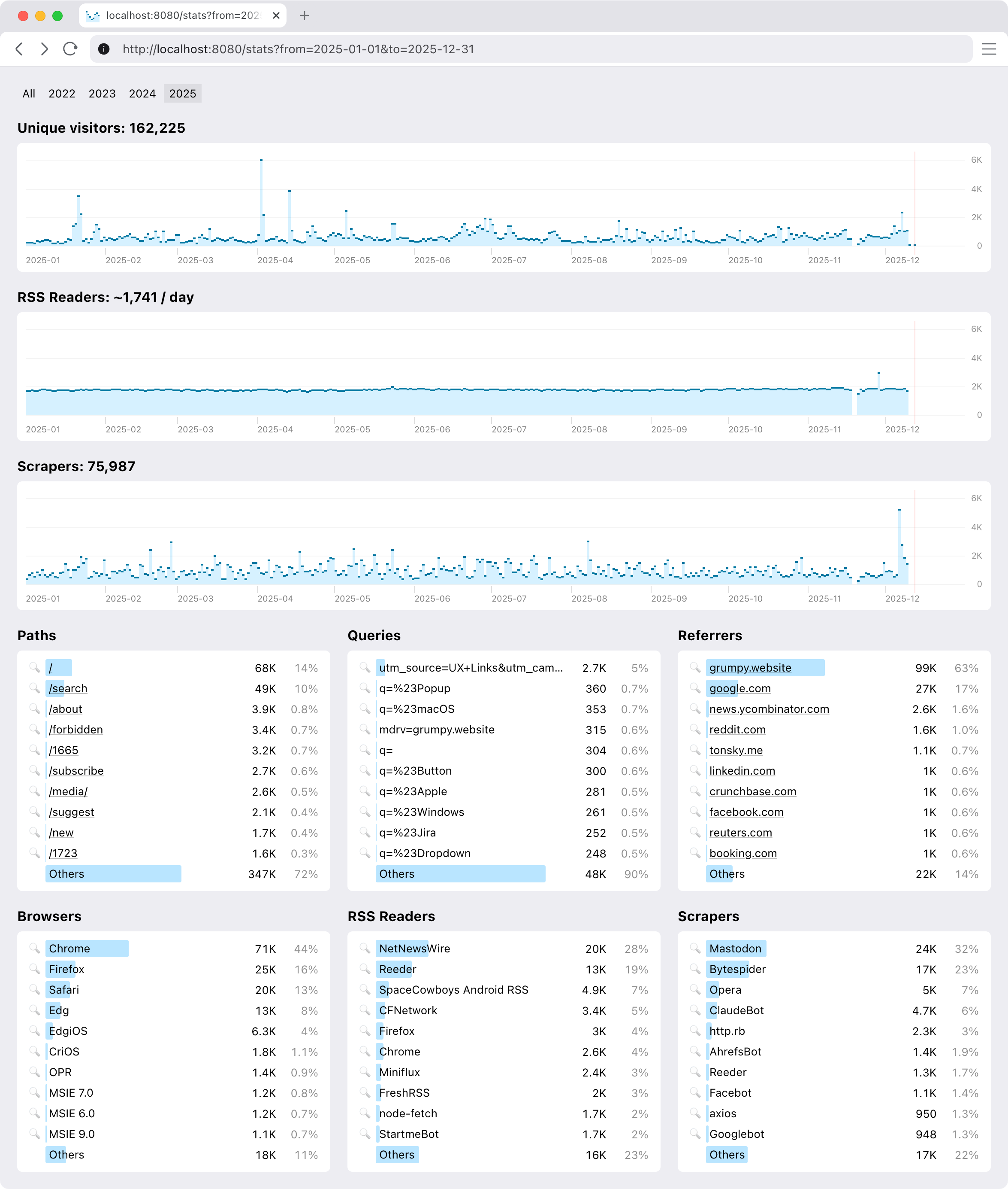
It’s pretty basic, but does a few things that were important to me.
Extremely easy to set up. And I mean it as a feature.
Just add our middleware to your Ring stack and get everything automatically: collecting and reporting.
(def app
  (-> routes
    ...
    (ring.middleware.params/wrap-params)
    (ring.middleware.cookies/wrap-cookies)
    ...
    (clj-simple-stats.core/wrap-stats))) ;; <-- just add this
It’s zero setup in the best sense: nothing to configure, nothing to monitor, minimal dependency. It starts to work immediately and doesn’t ask anything from you, ever.
See, you already have your web server, why not reuse all the setup you did for it anyway?
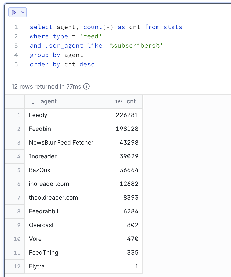
We distinguish between request types. In my case, I am only interested in live people, so I count them separately from RSS feed requests, favicon requests, redirects, wrong URLs, and bots. Bots are particularly active these days. Gotta get that AI training data from somewhere.
RSS feeds are live people in a sense, so extra work was done to count them properly. Same reader requesting feed.xml 100 times in a day will only count as one request.
Hosted RSS readers often report user count in User-Agent, like this:
Feedly/1.0 (+http://www.feedly.com/fetcher.html; 457 subscribers; like FeedFetcher-Google)

Mozilla/5.0 (compatible; BazQux/2.4; +https://bazqux.com/fetcher; 6 subscribers)

Feedbin feed-id:1373711 - 142 subscribers
My personal respect and thank you to everybody on this list. I see you.
Visualization is important, and so is choosing the correct graph type. This is wrong:

Continuous line suggests interpolation. It reads like between 1 visit at 5am and 11 visits at 6am there were points with 2, 3, 5, 9 visits in between. Maybe 5.5 visits even! That is not the case.
This is how a semantically correct version of that graph should look:

Some attention was also paid to having reasonable labels on axes. You won’t see something like 117, 234, 10875. We always choose round numbers appropriate to the scale: 100, 200, 500, 1K etc.
Goes without saying that all graphs have the same vertical scale and syncrhonized horizontal scroll.
We don’t offer much (as I don’t need much), but you can narrow reports down by page, query, referrer, user agent, and any date slice.
It would be nice to have some insights into “What was this spike caused by?”
Some basic breakdown by country would be nice. I do have IP addresses (for what they are worth), but I need a way to package GeoIP into some reasonable size (under 1 Mb, preferably; some loss of resolution is okay).
Finally, one thing I am really interested in is “Who wrote about me?” I do have referrers, only question is how to separate signal from noise.
Performance. DuckDB is a sport: it compresses data and runs column queries, so storing extra columns per row doesn’t affect query performance. Still, each dashboard hit is a query across the entire database, which at this moment (~3 years of data) sits around 600 MiB. I definitely need to look into building some pre-calculated aggregates.
One day.
Head to github.com/tonsky/clj-simple-stats and follow the instructions:

Let me know what you think! Is it usable to you? What could be improved?
P.S. You can try the live example at tonsky.me/stats. The data was imported from Nginx access logs, which I turned on and off on a few occasions, so it’s a bit spotty. Still, it should give you a general idea.
A Java Virtual Machine (JVM) é uma das tecnologias mais influentes e bem-sucedidas da história da computação moderna. Desde seu lançamento em 1995, a JVM tem sido fundamental para o sucesso da plataforma Java e representa um dos melhores exemplos de como abstrair a complexidade do hardware subjacente para fornecer portabilidade de código.
A JVM é uma máquina virtual que executa programas Java compilados em bytecode. Ela atua como uma camada de abstração entre o código Java e o sistema operacional/hardware subjacente, permitindo que o mesmo programa execute em diferentes plataformas sem modificações. Este é o princípio por trás do famoso lema "Write Once, Run Anywhere" (WORA) da linguagem Java.
É importante entender que a JVM não é apenas um interpretador de código Java. Ela é uma especificação completa que define como o bytecode deve ser executado, como a memória deve ser gerenciada, como threads devem funcionar e muitos outros aspectos fundamentais da execução de programas.
A arquitetura da JVM pode ser dividida em três componentes principais que trabalham em conjunto para executar aplicações Java.
O Class Loader é responsável por carregar arquivos de classe (.class) na memória da JVM. Este processo acontece em três fases distintas: carregamento, linkagem e inicialização.
Durante o carregamento, o Class Loader localiza e lê o arquivo .class correspondente, criando uma representação binária na memória. A fase de linkagem verifica se o bytecode está correto, prepara estruturas de dados para campos estáticos e resolve referências simbólicas para outras classes. Por fim, a inicialização executa construtores estáticos e inicializa variáveis estáticas.
O Class Loader funciona de forma hierárquica, com três níveis principais: Bootstrap ClassLoader (carrega classes do núcleo do Java), Extension ClassLoader (carrega extensões da plataforma) e Application ClassLoader (carrega classes da aplicação). Este mecanismo hierárquico permite isolamento e segurança ao carregar classes.
A JVM organiza a memória em várias áreas distintas, cada uma com propósito específico.
A Heap é onde todos os objetos são alocados. É a maior área de memória da JVM e é compartilhada entre todas as threads da aplicação. O Garbage Collector gerencia esta área, removendo objetos que não são mais referenciados. A heap é dividida em gerações (Young Generation, Old Generation) para otimizar a coleta de lixo.
A Method Area armazena metadados de classes, incluindo estruturas de classes, constantes de tempo de execução, código de métodos e construtores. Esta área também é compartilhada entre threads e contém o pool de constantes de tempo de execução.
A Stack é criada para cada thread e armazena frames de métodos. Cada frame contém variáveis locais, referências a operandos e informações sobre o método sendo executado. A stack segue o princípio LIFO (Last In, First Out).
O Program Counter Register mantém o endereço da instrução JVM sendo executada atualmente. Cada thread tem seu próprio PC register.
A Native Method Stack contém informações sobre métodos nativos (escritos em C/C++) utilizados pela aplicação através da Java Native Interface (JNI).
O Execution Engine é o componente que realmente executa o bytecode. Ele contém três elementos principais:
O Interpretador lê e executa instruções de bytecode uma por uma. Embora simples, a interpretação pura é lenta porque cada instrução precisa ser decodificada toda vez que é executada.
O JIT Compiler (Just-In-Time Compiler) melhora drasticamente a performance ao compilar bytecode frequentemente executado diretamente para código de máquina nativo. O código compilado é armazenado em cache e executado diretamente pelo processador, eliminando a overhead de interpretação. O JIT usa técnicas sofisticadas de otimização, incluindo inlining de métodos, eliminação de código morto e otimizações específicas do processador.
O Garbage Collector gerencia automaticamente a memória, identificando e removendo objetos que não são mais acessíveis. Existem vários algoritmos de GC disponíveis, cada um otimizado para diferentes cenários de uso.
Quando você executa um programa Java, uma sequência complexa de eventos ocorre:
Primeiro, o código-fonte Java (.java) é compilado pelo compilador javac em bytecode (.class). Este bytecode é independente de plataforma e contém instruções que a JVM pode entender.
Quando você inicia a aplicação, a JVM é inicializada e o Class Loader começa a carregar as classes necessárias, começando pela classe principal que contém o método main. As classes são carregadas sob demanda (lazy loading), não todas de uma vez.
O bytecode é inicialmente interpretado, mas o JIT Compiler monitora quais partes do código são executadas com frequência (hot spots). Esses hot spots são compilados para código nativo e armazenados em cache, melhorando significativamente a performance em execuções subsequentes.
Durante toda a execução, o Garbage Collector monitora a heap, identificando objetos que não têm mais referências e liberando sua memória automaticamente.
O Garbage Collection (GC) é um dos recursos mais importantes da JVM, liberando desenvolvedores da tarefa complexa e propensa a erros de gerenciar memória manualmente.
O GC opera identificando quais objetos na heap ainda são acessíveis (alcançáveis através de referências) e quais não são. Objetos não alcançáveis são considerados "lixo" e podem ser removidos.
O processo começa com um conjunto de raízes (GC roots), que incluem variáveis locais em stacks de threads, campos estáticos de classes e referências JNI. A partir dessas raízes, o GC traça um grafo de todas as referências, marcando objetos alcançáveis.
A heap é dividida em gerações baseadas no princípio de que a maioria dos objetos tem vida curta:
A Young Generation é onde novos objetos são alocados. Ela é subdividida em Eden (onde objetos são criados inicialmente) e dois espaços Survivor. Quando Eden fica cheio, ocorre um Minor GC que move objetos sobreviventes para um espaço Survivor.
A Old Generation contém objetos que sobreviveram a vários ciclos de GC na Young Generation. Coletas aqui (Major GC ou Full GC) são menos frequentes mas levam mais tempo.
A Metaspace (substituiu a Permanent Generation no Java 8) armazena metadados de classes e não é tecnicamente parte da heap gerenciada.
A JVM oferece vários coletores de lixo, cada um otimizado para diferentes cenários:
O Serial GC usa uma única thread e é adequado para aplicações pequenas com heaps de até alguns megabytes.
O Parallel GC usa múltiplas threads para coleta, maximizando throughput mas com pausas perceptíveis. É o padrão em muitas versões da JVM.
O CMS (Concurrent Mark Sweep) executa a maior parte do trabalho de coleta concorrentemente com threads da aplicação, minimizando pausas. Foi descontinuado em versões recentes do Java.
O G1 GC (Garbage First) divide a heap em regiões e prioriza a coleta de regiões com mais lixo. Oferece pausas previsíveis e é o padrão desde o Java 9.
O ZGC e Shenandoah são coletores de baixa latência que mantêm pausas abaixo de 10ms mesmo com heaps de terabytes, usando técnicas avançadas de coloração de ponteiros e compactação concorrente.
O JIT Compiler é fundamental para a performance da JVM, transformando bytecode em código nativo otimizado durante a execução.
A JVM moderna usa compilação em camadas (tiered compilation), combinando interpretação com dois níveis de compilação JIT:
O C1 Compiler compila código rapidamente com otimizações básicas, ideal para código executado poucas vezes ou durante inicialização.
O C2 Compiler realiza otimizações agressivas mas leva mais tempo para compilar. É usado para hot spots que são executados muitas vezes.
O JIT aplica várias otimizações sofisticadas:
Inlining substitui chamadas de métodos pelo corpo do método, eliminando a overhead de chamada e permitindo otimizações adicionais.
Escape Analysis determina se objetos podem ser alocados na stack ao invés da heap, reduzindo pressão no GC.
Loop Unrolling desenrola loops, reduzindo a overhead de controle de loop e permitindo melhor paralelização.
Dead Code Elimination remove código que nunca será executado, reduzindo o tamanho do código compilado.
Branch Prediction otimiza condicionais baseado em padrões de execução observados.
Um aspecto único do JIT é a capacidade de desotimizar código. Se as suposições usadas durante otimização se tornam inválidas (por exemplo, uma classe que era final é substituída por herança), a JVM pode reverter para bytecode interpretado ou recompilar com suposições diferentes.
A JVM oferece centenas de parâmetros de configuração para otimizar performance para diferentes cenários de uso.
Os parâmetros mais comuns controlam o tamanho da heap:
-Xms define o tamanho inicial da heap, enquanto -Xmx define o tamanho máximo. Definir ambos com o mesmo valor evita redimensionamento durante execução.
-XX:NewRatio controla a proporção entre Young e Old Generation. Um valor de 2 significa que Old Generation é duas vezes maior que Young Generation.
-XX:SurvivorRatio define a proporção entre Eden e espaços Survivor na Young Generation.
-XX:+UseSerialGC, -XX:+UseParallelGC, -XX:+UseG1GC, -XX:+UseZGC selecionam diferentes coletores de lixo.
Para G1, -XX:MaxGCPauseMillis define um objetivo de tempo de pausa máximo.
-XX:CompileThreshold define quantas vezes um método deve ser executado antes de ser compilado pelo JIT.
-XX:+TieredCompilation habilita compilação em camadas (habilitado por default em JVMs modernas).
Entender o comportamento da JVM em tempo de execução é crucial para diagnosticar problemas e otimizar performance.
JVMTI é uma interface nativa que permite ferramentas externas inspecionar e controlar a JVM. Profilers, debuggers e ferramentas de monitoramento usam JVMTI.
jps lista processos Java em execução no sistema.
jstat monitora estatísticas da JVM, incluindo uso de heap, contadores de GC e compilação JIT.
jmap gera heap dumps e histogramas de objetos na memória.
jstack captura stack traces de todas as threads, útil para diagnosticar deadlocks.
jcmd é uma ferramenta unificada que combina funcionalidade de várias ferramentas.
VisualVM fornece uma interface gráfica para monitoramento, profiling e análise de heap dumps.
Java Mission Control oferece análise avançada de performance usando Java Flight Recorder (JFR), que coleta dados de diagnóstico com overhead mínimo.
Embora a JVM seja uma especificação, existem várias implementações diferentes:
HotSpot é a implementação de referência da Oracle, usada na maioria das instalações Java. O nome vem de sua capacidade de identificar hot spots no código.
OpenJ9 da Eclipse Foundation é focada em eficiência de memória e tempo de inicialização rápido.
GraalVM é uma JVM moderna que suporta múltiplas linguagens e permite compilação ahead-of-time (AOT) para executáveis nativos.
Azul Zing é uma JVM comercial otimizada para baixa latência com o coletor de lixo C4 (Continuously Concurrent Compacting Collector).
A JVM não executa apenas Java. Muitas outras linguagens compilam para bytecode JVM:
Kotlin é uma linguagem moderna que adiciona recursos como null-safety, funções de extensão e corrotinas.
Scala combina programação funcional e orientada a objetos com um poderoso sistema de tipos.
Groovy é uma linguagem dinâmica com sintaxe concisa, popular para scripts e DSLs.
Clojure é um dialeto moderno de Lisp focado em programação funcional e imutabilidade.
Todas essas linguagens se beneficiam do ecossistema Java, incluindo bibliotecas, ferramentas e otimizações da JVM.
Apesar de suas muitas vantagens, a JVM tem algumas limitações:
O tempo de inicialização pode ser significativo porque a JVM precisa carregar classes, inicializar subsistemas e permitir que o JIT compile código quente. Isso é problemático para aplicações serverless.
O consumo de memória base da JVM é considerável, incluindo memória para metadados de classes, código compilado e estruturas internas.
O GC pause pode causar latências imprevisíveis, embora coletores modernos como ZGC minimizem isso.
A compilação AOT limitada historicamente impediu otimizações em tempo de build, embora projetos como GraalVM Native Image estejam mudando isso.
A JVM continua evoluindo para atender às necessidades modernas:
Project Loom introduz threads virtuais (fibras) para concorrência massiva com baixo overhead.
Project Panama melhora a interoperabilidade com código nativo, facilitando chamadas a bibliotecas C/C++.
Project Valhalla adiciona tipos de valor (value types) que combinam benefícios de primitivos e objetos.
Project Leyden foca em melhorar tempo de inicialização e reduzir consumo de memória através de compilação AOT e otimizações de tempo de build.
A JVM é uma peça fundamental da infraestrutura de software moderna, executando incontáveis aplicações críticas em todo o mundo. Sua combinação de portabilidade, gerenciamento automático de memória e otimizações de performance sofisticadas a tornam uma plataforma excepcional para desenvolvimento de software.
Compreender os internals da JVM - desde o class loading até garbage collection e compilação JIT - permite que desenvolvedores escrevam código mais eficiente, diagnostiquem problemas de performance e façam decisões arquiteturais mais informadas.
A evolução contínua da JVM através de projetos inovadores garante que ela permanecerá relevante e competitiva nos próximos anos, adaptando-se a novos paradigmas de computação como containers, serverless e aplicações de baixa latência.
Para qualquer desenvolvedor trabalhando no ecossistema Java, investir tempo em entender profundamente a JVM é um dos melhores investimentos que se pode fazer para o crescimento profissional.
Driving Plotly to Update a Chart with New Points.
This is the second part of our Machine Learning in Clojure with libpython‑clj series. If you missed Series 1, we covered how Clojure can use Python’s ML libraries through libpython‑clj. In this article, we focus on Bayesian Networks. We will show how to train them, run queries, and use them in Clojure.
Machine learning is not only for Python. With libpython‑clj, Clojure teams can use PyMC, scikit‑learn, and pgmpy. And they can keep the JVM and the functional style they like. The aim is simple: make ML in Clojure clear, practical, and ready for production.
Bayesian Networks are good when you need clarity. They model uncertainty. They use domain knowledge. And they answer “what if?” questions without guesswork.
➤ Small to medium datasets.
➤ Compliance‑heavy work in healthcare, finance, and logistics.
➤ When explainability is required.
This walkthrough builds a simple BN in Python. Then run it from Clojure using libpython‑clj. The process is clear.
Flexiana is a Clojure consultancy. We help teams connect Clojure and ML in real projects. We share code, write about patterns, and ship systems that are easy to reason about. If you need support with interop, pipelines, or interpretable models, we are a solid partner.
“Bayesian reasoning helps teams make better calls in logistics, healthcare, and fintech. With Clojure’s REPL and Python’s ML tools, you move faster and stay confident.” – Flexiana ML Team
A Bayesian Network is a directed acyclic graph. Each node is a random variable. Each edge shows how one variable depends on another. The graph encodes conditional probabilities that describe how events influence each other.
Bayesian Networks are not just about guessing what will happen next. They show why something is likely or not, based on how the graph’s parts connect. When you are dealing with uncertainty, these networks give you both a prediction and a peek behind the curtain.
| Aspect | Bayesian Networks (BNs) | Neural Networks (NNs) |
|---|---|---|
| Structure | Graph with variables | Layers with neurons/weights |
| Nodes | Variables with probabilities | Units with weights + activations |
| Edges | Show dependencies | Pass signals between neurons |
| Flow of Information | Probabilities through a graph | Numbers through weighted sums |
| Interpretability | Clear, easy to trace | Often, a black box |
| Data Needs | Small datasets + domain knowledge | Large datasets needed |
| Strengths | Model uncertainty, “what if?” | Finds patterns in complex data |
| Limitations | Weak with high‑dimensional data | Hard to explain the reasoning |
Neural Networks (NNs) really stand out for image recognition, speech, and other messy, unstructured data. They work best with huge datasets and find hidden patterns.
Bayesian Networks fit different needs:
➤ When datasets are smaller, but domain knowledge is strong
➤ When decisions must be explained to stakeholders
➤ When uncertainty needs to be modelled clearly
With all these considered, Neural Networks find hidden patterns. Bayesian Networks help with clarity, reasoning, and trust.
You can actually see how Bayesian Networks think. Every variable and every link is there in the graph. So if something happens, you can trace the whole path back and explain it. That is a big deal in places like healthcare or finance, where you have to tell regulators or your team exactly why a decision was made. With Neural Networks, they usually keep that logic hidden, which just isn’t good enough when you need transparency.
Bayesian Networks handle uncertainty directly. They do not just return one answer but give you probabilities, so you know what might happen and what’s not, and how sure the model is. That helps when your data is messy or incomplete. Neural Networks, on the other hand, usually just pick one outcome, which can be misleading when things are not clear.
Bayesian Networks can include domain knowledge. You can turn relationships and rules from the real world into edges and probability tables. This keeps the model grounded, especially when you do not have a ton of data. Neural Networks, on the other hand, need huge datasets to learn patterns and are not great at encoding expert rules.
PyMC Labs recently pointed out that “Bayesian modelling is really shaping business decisions these days. Probabilistic forecasting models are popping up all over the place- in retail, finance, energy, you name it. Businesses are leaning into these approaches more and more”.
Flexiana focuses on interpretable ML for compliance‑heavy work. Our projects lean on clear reasoning and stable interoperability. Pairing Clojure’s functional style with BN reasoning helps teams build systems that are practical and explainable.
➤ “What if?” analysis: If a shipment is delayed, what is the churn risk? BNs model scenarios and return clear probabilities.
➤ Small or medium datasets: Expert knowledge– Encode known relationships directly. Useful when data is limited.
➤ Compliance‑heavy industries: Interpretable reasoning– Show why an outcome is likely. Fits healthcare, finance, and logistics.
➤ Flexiana case mentioned: Decision support– Flexiana has used BNs for logistics and healthcare clients. The focus is on clear reasoning and compliance‑friendly workflows.
➤ High‑dimensional inputs: Images and audio involve thousands of features. BNs struggle at this scale.
➤ Unstructured data: Text, images, and raw audio need feature extraction. Deep learning handles this better.
➤ Arbitrary function approximation: Neural Networks capture complex, nonlinear patterns. BNs are built for probabilistic reasoning, not every function shape.
Here’s a basic example with pgmpy, a Python library. It builds a small Bayesian Network with two nodes and one dependency.
from pgmpy.models import BayesianNetwork
from pgmpy.factors.discrete import TabularCPD

# Define the network structure
model = BayesianNetwork([('Rain', 'Traffic')])

# Define the CPDs (Conditional Probability Distributions)
cpd_rain = TabularCPD(
    variable='Rain',
    variable_card=2,
    values=[[0.7], [0.3]]  # 70% no rain, 30% rain
)

cpd_traffic = TabularCPD(
    variable='Traffic',
    variable_card=2,
    values=[
        [0.9, 0.4],  # Probability of no traffic
        [0.1, 0.6]   # Probability of traffic
    ],
    evidence=['Rain'],
    evidence_card=[2]
)

# Add CPDs to the model
model.add_cpds(cpd_rain, cpd_traffic)

# Check if the model is valid
print(model.check_model())
What this does:
➤ Builds a BN with two variables: Rain and Traffic.
➤ Shows that rain raises the chance of traffic
➤ Checks that the model and probabilities are valid
For more details, check the official documentation:
➤ Train in Python: Build and check the BN with pgmpy or PyMC.
➤ Load via libpython‑clj: Import the Python model into Clojure.
➤ Wrap inference in Clojure: Write small functions for queries and “what if?” checks.
Clojure code snippet
(ns bn.interop
  (:require [libpython-clj2.python :as py]
            [libpython-clj2.require :refer [require-python]]))

(require-python '[pgmpy.models :as models])
(require-python '[pgmpy.factors.discrete :as factors])

(defonce ^:private py-sys (py/initialize!))

;; Load a trained BN (assume serialized or constructed via Python)
(def model
  (models/BayesianNetwork [["Rain" "Traffic"]]))

;; Example: set CPDs (normally loaded from Python artifacts)
(def cpd-rain
  (factors/TabularCPD
   "Rain" 2
   (py/list [[0.7] [0.3]])))

(def cpd-traffic
  (factors/TabularCPD
   "Traffic" 2
   (py/list [[0.9 0.4]
             [0.1 0.6]])
   :evidence (py/list ["Rain"])
   :evidence_card (py/list [2])))

(.add_cpds model cpd-rain cpd-traffic)

(defn prob-traffic
  "Return P(Traffic | Rain = state). state: 0=no rain, 1=rain."
  [state]
  ;; Placeholder for actual inference call
  (case state
    0 {:no-traffic 0.9 :traffic 0.1}
    1 {:no-traffic 0.4 :traffic 0.6}))
➤ Enterprise JVM focus: Flexiana’s tutorials show how to bridge Python ML with Clojure in enterprise JVM stacks. The focus is clear interop, stable deployment, and explainable models.
➤ Utility functions for boxed math: Avoid unnecessary boxing. Use primitives where possible and keep Python calls lean.
➤ Batch calls for efficiency: Run queries in groups to cut overhead.
➤ Caching strategies: Cache fixed CPDs and reuse common results. Memoize repeated “what if?” checks.

Bayesian networks are great for running “what if?” modeling in logistics. If a shipment gets delayed, these models help you see the chances of supplier bottlenecks, missed deliveries, or even losing customers. Managers do not have to guess; they get clear numbers and can actually plan around them.
➤ Use case: You can map out how a delay might lead to customer churn, or spot risks up and down the supply chain.
➤ Output: You can hand these probabilities to your ops or finance teams and actually explain what’s behind them.
➤ Value: You get smarter backup plans and fewer surprises.

BNs connect symptoms, test results, and conditions, showing how each piece of information changes the probabilities of a diagnosis. The reasoning is not hidden- clinicians can see not just what the model predicts, but how sure it is.
➤ Use case: If you plug in a set of symptoms, you get a clear picture of which conditions are most likely.
➤ Output: The logic stays out in the open, so anyone reviewing the case can follow every step.
➤ Value: This kind of transparency is good when you need to explain decisions or meet strict compliance rules.
Employing Bayesian Networks for the Diagnosis and Prognosis of Diseases: A Comprehensive Review (arXiv, 2023) – This paper gives an overview of how Bayesian Networks support medical diagnosis and prognosis. It shows how they use medical knowledge and manage uncertainty in decisions.
BNs do not just spot fraud- they break down what made a transaction suspicious in the first place. You get to see exactly which factors raised the red flag, not just a vague alert. That kind of clarity makes audits and regulator checks way smoother.
➤ Use case: They scan transaction patterns and highlight the risky ones.
➤ Output: Real reasons for every alert, not just a score.
➤ Value: You end up with detection you can actually trust and clearer investigations.
According to a 2025 industry survey, more than 70% of financial firms have adopted probabilistic or machine learning models to detect fraud, reflecting a clear shift away from rule‑based systems.
➤ Faster orchestration and deployment: For starters, you can move fast. The REPL lets you test ideas and make changes quickly, so updates are faster without waiting around for long builds.
➤ Seamless JVM integration: Clojure integrates nicely with the JVM. You can plug ML models right into your current systems. No need for extra layers or awkward workarounds.
➤ Lower barrier for Clojure teams: if your team already knows Clojure, you do not have to rebuild your stack or retrain everyone just to bring machine learning into the picture. You get to use the tools you know, and still take advantage of ML.
Explore Flexiana’s consulting to fit ML into your Clojure stack. Interop, deployment, and compliance‑friendly workflows: that’s the focus.
# Example using pgmpy
# pip install pgmpy

from pgmpy.models import BayesianNetwork
from pgmpy.factors.discrete import TabularCPD
from pgmpy.inference import VariableElimination

# 1) Structure: Smoking -> Cancer, and Pollution -> Cancer
model = BayesianNetwork([
    ('Smoking', 'Cancer'),
    ('Pollution', 'Cancer')
])

# 2) CPDs
cpd_smoking = TabularCPD(
    variable='Smoking',
    variable_card=2,
    values=[[0.6], [0.4]],  # P(Smoking=no)=0.6, P(Smoking=yes)=0.4
    state_names={'Smoking': ['no', 'yes']}
)

cpd_pollution = TabularCPD(
    variable='Pollution',
    variable_card=2,
    values=[[0.7], [0.3]],  # P(Pollution=low)=0.7, P(Pollution=high)=0.3
    state_names={'Pollution': ['low', 'high']}
)

# Cancer depends on Smoking and Pollution
cpd_cancer = TabularCPD(
    variable='Cancer',
    variable_card=2,
    values=[
        # Cancer = no
        [0.99, 0.97, 0.95, 0.90],
        # Cancer = yes
        [0.01, 0.03, 0.05, 0.10]
    ],
    evidence=['Smoking', 'Pollution'],
    evidence_card=[2, 2],
    state_names={
        'Cancer': ['no', 'yes'],
        'Smoking': ['no', 'yes'],
        'Pollution': ['low', 'high']
    }
)

# 3) Attach CPDs and check model
model.add_cpds(cpd_smoking, cpd_pollution, cpd_cancer)
assert model.check_model()

# 4) Inference
infer = VariableElimination(model)

# P(Cancer | Smoking=yes, Pollution=high)
q = infer.query(
    variables=['Cancer'],
    evidence={'Smoking': 'yes', 'Pollution': 'high'}
)
print(q)  # Prints distribution for Cancer=no/yes

# P(Smoking | Cancer=yes)
q2 = infer.query(
    variables=['Smoking'],
    evidence={'Cancer': 'yes'}
)
print(q2)
➤ Structure: A clear DAG with three variables; Cancer has two parents.
➤ Nodes: Random variables with named states.
➤ Edges: Smoking and Pollution feed into Cancer.
➤ CPDs: Tables capture prior knowledge and uncertainty.
➤ Inference: Use variable elimination for “what if?” queries.
This example uses libpython‑clj to import pgmpy, set up the network, and run queries in Clojure.
;; deps.edn
;; {:deps {clj-python/libpython-clj {:mvn/version "2.024"}}
;;  :paths ["src"]}

(ns bn.example
  (:require
   [libpython-clj2.python :as py]
   [libpython-clj2.require :refer [require-python]]))

;; Initialize Python
(py/initialize!)

;; Require Python packages
(require-python '[pgmpy.models :as models])
(require-python '[pgmpy.factors.discrete :as factors])
(require-python '[pgmpy.inference :as inf])

(defn build-model []
  ;; 1) Structure
  (let [model (models/BayesianNetwork
               [(py/tuple "Smoking" "Cancer")
                (py/tuple "Pollution" "Cancer")])]

    ;; 2) CPDs
    (def cpd-smoking
      (factors/TabularCPD
       :variable "Smoking"
       :variable_card 2
       :values (py/list [(py/list [0.6])
                          (py/list [0.4])])
       :state_names (py/dict {"Smoking" (py/list ["no" "yes"])})))

    (def cpd-pollution
      (factors/TabularCPD
       :variable "Pollution"
       :variable_card 2
       :values (py/list [(py/list [0.7])
                          (py/list [0.3])])
       :state_names (py/dict {"Pollution" (py/list ["low" "high"])})))

    (def cpd-cancer
      (factors/TabularCPD
       :variable "Cancer"
       :variable_card 2
       :values (py/list [(py/list [0.99 0.97 0.95 0.90])   ;; Cancer = no
                          (py/list [0.01 0.03 0.05 0.10])]) ;; Cancer = yes
       :evidence (py/list ["Smoking" "Pollution"])
       :evidence_card (py/list [2 2])
       :state_names (py/dict {"Cancer" (py/list ["no" "yes"])
                              "Smoking" (py/list ["no" "yes"])
                              "Pollution" (py/list ["low" "high"])})))

    ;; 3) Attach CPDs
    (.add_cpds model cpd-smoking cpd-pollution cpd-cancer)

    ;; 4) Sanity check
    (assert (.check_model model))
    model))

(def model (build-model))
(def infer (inf/VariableElimination model))

;; Query: P(Cancer | Smoking=yes, Pollution=high)
(def cancer-q
  (.query infer
          (py/list ["Cancer"])
          :evidence (py/dict {"Smoking" "yes"
                              "Pollution" "high"})))

(println cancer-q)

;; Query: P(Smoking | Cancer=yes)
(def smoking-q
  (.query infer
          (py/list ["Smoking"])
          :evidence (py/dict {"Cancer" "yes"})))

(println smoking-q)
Interop flow:
➤ Build: Mirror the Python BN and CPDs with libpython‑clj.
➤ Infer: Call pgmpy’s VariableElimination from Clojure.
➤ Return: Get Python objects, then print or convert to Clojure data.
(defn dist->map [python-factor]
  ;; Converts pgmpy DiscreteFactor result into a Clojure map of state->prob
  (let [vars   (vec (py/get-attr python-factor "variables"))
        states (vec (py/call-attr python-factor "state_names" (first vars)))
        values (vec (py/call-attr python-factor "values"))]
    (zipmap states values)))

(println (dist->map cancer-q))
(println (dist->map smoking-q))
Label conversion: Map states to values, e.g., {“no” 0.90, “yes” 0.10}.
Engagement tip: Log queries and results to show stakeholders how each node shapes outcomes.
Not at all. Neural Networks learn patterns from tons of data, while Bayesian Networks focus on cause and effect, mapping out probabilities and showing you how they conclude.
Honestly, they are not built for that. Bayesian Networks help with small or medium datasets, especially when you need expert input. If you have massive, unstructured data, deep learning usually does a better job.
Clojure runs on the JVM, so it fits right into enterprise setups. Plus, if you need something from Python, you can just call those libraries- no need to pick one or the other.
It makes things easy. Clojure can import Python ML libraries directly- train your model in Python, then query it from Clojure. No need to build complicated bridges between the two.
Healthcare, finance, and logistics rely on Bayesian models. They want explainable results, clear probabilities, and the ability to test out “what if?” scenarios quickly.
Machine learning in Clojure is practical for real teams. With libpython‑clj, you can use Python’s ML libraries while staying in the JVM stack you already trust. That means faster iteration, smoother deployment, and less friction for Clojure developers.
Bayesian Networks add clear value. They do not just predict; they show the reasoning. This matters in healthcare, finance, and logistics, where decisions carry weight. BNs handle uncertainty and map cause‑and‑effect, so managers and auditors can see why a result makes sense.
If your team is exploring ML in Clojure, now is a good time to try it. Share your thoughts, compare notes, and check the sample code in our GitHub repo.
If you want help, Flexiana’s consulting team can guide design, deployment, and integration so it fits your stack.
The post Machine Learning in Clojure with libpython‑clj: Using Bayesian Networks for Smarter, Interpretable AI [Series 2] appeared first on Flexiana.
Code
;; map_ops.clj

(defn maps-op ([func map-1 map-2 default-value]
               (let [map-1-keys (keys map-1)
                     map-2-keys (keys map-2)
                     keys (distinct (concat map-1-keys map-2-keys))]
                 (->> (map #(assoc {} %
                                   (func
                                    (get map-1 % default-value)
                                    (get map-2 % default-value))) keys)
                      (apply merge))))
  ([func map-1 map-2]
     (maps-op func map-1 map-2 nil)))

(defn map-op
  ([func map-1]
   (let [keys (keys map-1)]
     (->> (map #(assoc {} %
                       (func
                        (get map-1 %))) keys)
          (apply merge))))
  ([func m val]
   (maps-op func m {} val)))

(maps-op + {:a 1 :b 2 :c 5} {:a 3 :b 4} 0)
;;=> {:a 4, :b 6, :c 5}

(maps-op + {:a 1 :b 2} {:a 3 :b 4})
;;=> {:a 4, :b 6}

(map-op + {:a 1 :b 2 :c 5} 5)
;;=> {:a 6, :b 7, :c 10}

(map-op inc {:a 1 :b 2 :c 5})
;;=> {:a 2, :b 3, :c 6}

;; how it works

(def map-1 {:a 1 :b 2})
(def map-2 {:a 3 :b 4})

(def map-1-keys (keys map-1))

map-1-keys
;;=> (:a :b)

(def map-2-keys (keys map-2))

map-2-keys
;;=> (:a :b)

(distinct (concat map-1-keys map-2-keys))
;;=> (:a :b)

(+ (get map-1 :a) (get map-2 :a))
;;=> 4

(assoc {} :a
       (+ (get map-1 :a) (get map-2 :a)))

;;=> {:a 4}

(def func +)

(map #(assoc {} %
              (func
               (get map-1 %)
               (get map-2 %))) '(:a :b))
;;=> ({:a 4} {:b 6})

(merge {:a 4} {:b 6})
;;=> {:a 4, :b 6}

(apply merge [{:a 4} {:b 6}])
;;=> {:a 4, :b 6}
Pixelation is everywhere these days, from retro game aesthetics to modern design trends. But if you've ever tried to create pixel art from a photograph, you've probably noticed that the results often look a bit off. Edges get jagged, important features get distorted, and the whole image tends to lose its character.
Most pixelation algorithms rely on the same approach of downscaling the image, then upscaling it back. While this is fast and cheap to implement, it treats every part of the image the same way forcing a rigid grid that cuts indiscriminately across edges, faces, and fine details.
In this post, we'll take a look at a strategy of using edge-aware pixelation. The idea here is to use an algorithm that adapts to the structure of the image rather than forcing a uniform grid onto it. We'll look at how it works, why it tends to produce better results, and the trade-offs involved.
Let's start by looking at what most pixelation libraries do under the hood. The most common approach uses standard image scaling with smoothing.
// Pseudo-code for traditional pixelation
const downscaled = scaleDown(image, pixelSize); // Uses bilinear/bicubic
const pixelated = scaleUp(downscaled, originalSize); // Nearest-neighbor
While this works, there are a few obvious problems. Smoothing filters tend to blur important edges before downsampling, and the pixel grid doesn't care about the image content. This often leads to artifacts where edges get "chopped" across pixel boundaries, creating jagged lines. You also end up losing fine features like eyes or text.
Some approaches try to improve on this using median color sampling instead of averaging.
// Sample colors in each block, pick median
const blockColor = median(colorsInBlock);
This avoids some of the blurring, but it still suffers from the same fixed grid issue. It ignores the image structure and can create harsh transitions between blocks.
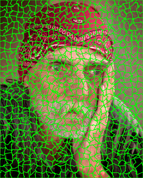
Basically, all these methods force a uniform grid onto the image without considering its content. The result is usually pixel blocks that cut across important features. For example, if we use the following image from wikimedia as the input.

The result ends up looking something like the following when using a naive pixelation algorithm:
![]()
Instead of forcing a rigid grid, we can let the grid adapt to the image. This is the core idea behind edge-aware pixelation. We can treat pixelation as an optimization problem with four main stages.
First, we need to understand where the important features are in the image.
// Sobel operators detect gradient magnitude and direction
const gradient = calculateGradient(image);
const edges = applyNonMaximumSuppression(gradient);
const edgeMap = thresholdEdges(edges, sharpness);
We use Sobel operators to compute the gradient magnitude, and then apply non-maximum suppression to thin the edges to a single-pixel width. Finally, we use percentile-based thresholding to adapt to the edge distribution of the specific image. Since this can be computationally expensive, using WebGL can provide a significant speedup here.
This gives us an edge map where bright pixels represent edges and dark pixels represent smooth regions.

Next, we start with a regular grid matching the target pixel size.
const grid = createUniformGrid(width, height, pixelSize);
Unlike traditional methods, the grid is just a starting point. Each cell is defined by four corner points which we can move around.

This is where the actual work happens. We iteratively move the grid corners to align the cell boundaries with the detected edges.
for (let iteration = 0; iteration < numIterations; iteration++) {
  for (each corner in grid) {
    // Search nearby positions
    const candidates = searchNeighborhood(corner, stepSize);

    // Evaluate how well each position aligns edges
    for (const candidate of candidates) {
      const score = evaluateEdgeAlignment(candidate, edgeMap);
      if (score > bestScore) {
        bestPosition = candidate;
      }
    }

    // Move corner toward best position (with damping)
    corner.moveToward(bestPosition, damping);
  }
}
For each corner, we test multiple positions in a local neighborhood and evaluate the alignment by sampling edge strength along the grid edges. We want to find positions where the grid boundaries follow the edges continuously. We also use damping to prevent over-optimization and maintain stability.
The result is a grid that bends and adapts to align with the natural structure of the image.
Finally, we need to assign colors to our optimized cells.
for (each cell in grid) {
  const pixels = samplePixelsInCell(cell);

  // Blend between average (soft) and median (crisp) based on edge presence
  if (cell.hasEdges) {
    color = blend(average(pixels), median(pixels), sharpness);
  } else {
    color = average(pixels); // Smooth regions use average
  }

  renderCell(cell, color);
}
Here we can use a blending strategy. For smooth regions, we use the average color for natural blending. For edge regions, we can blend between average and median based on the desired sharpness. This lets us tune the aesthetic from soft, blended edges to crisp, high-contrast ones. Looking at the two methods side by side, we can see how much smoother the resulting image is:
| Edge detection | Naive |
|---|---|
There are several advantages to this approach. The most obvious is edge preservation. Traditional methods create jagged artifacts because pixel boundaries cut across edges. By aligning the grid boundaries with the edges, we can preserve continuity and create smoother transitions.
This also means we don't get those choppy edges on outlines, and we can preserve fine details like facial features or text much better. The algorithm effectively has some semantic awareness of what's important in the image.
However, there are trade-offs to consider. The adaptive grid and color blending can produce softer edges compared to traditional methods. If you're looking for extremely crisp, high-contrast pixel art with hard edges, like what you'd see in retro games, traditional downsampling might actually be a better fit.
You also get less contrast in some cases. The color blending can reduce the overall "punchiness" compared to median sampling.
Performance is another factor. Edge-aware pixelation is computationally more intensive. You have to handle edge detection, iterative grid optimization, and spatial hashing for rendering. While WebGL optimizations make it practical taking 100-500ms on most images, simple downsampling will always be faster.
I've found that edge-aware pixelation works best for photographs, portraits, and complex scenes where preserving structure is important. It's less ideal for abstract art or images where a uniform grid is desired for stylistic reasons.
By detecting edges and optimizing alignment, edge-aware pixelation produces pixel art that does a good job of preserving the essence of the original while still achieving low-resolution aesthetic.
If you're interested in trying this out live here, and all the code is available as an open source library called Pixel Mosaic that implements both traditional and edge-aware pixelation.
I hope this gives you some ideas for your own image processing projects. Sometimes the simple method is enough, but for complex images, the extra effort of edge-aware processing can be well worth it.
Besides updating the About page, I wanted to start writing again about the various tools and solutions I’m using more frequently. Lately, the tools are more in the physical realm than in software. (But I will note here, that 2025 is finally the year that I switched to neovim for myself instead of vim. More on this at the end of the list.)
I’ve tried carrying EDC pocket knives for opening boxes, and I’ve tried stocking cheap scissors in drawers all over the house. In the end, the best way to open boxes turns out to be these ceramic-bladed box openers from Slice. The blades aren’t sharp enough to cut a finger, but they will open tape, including that tricky tape that has threads in it. When you let go, the blade retracts, and can’t poke you when you reach into a pocket or a drawer. It sounds basic, but given how much I get shipped to me for convenience, this has been one of my top tools for the last few years.

I try to fix things myself when I can. If you DIY stuff, you’ve probably run into this problem: screws like to roll off surfaces and disappear. I got tired of this, and since most screws are made from ferrous metal, these little magnetic parts bowls solve the problem for me. I’ve got a few upstairs near where I practice guitar and where my home office desk is, and a few more downstairs on my work bench. Conveniently, the magnet in the base will also make the bowl stick to anything iron or steel, too, so I tend to be able to “plunk” down a bowl on something like a desk frame or my work bench vise, and know that all the screws for a project will stay in there. (Provided they’re ferrous.) Compared to random jars or recycled plastic dishes full of screws, this feels like a big upgrade for me, and so that is why this item is second on my list for 2025. There’s lots of variations of these available online or at your local stores – I recommend trying to find them in the local hardware store.

Even with several complete small screwdriver sets and an electric drill that can fit screwdriver bits, I wanted something small that I could keep in my office and use for screwdriver tasks. I imagined it could help with taking apart keyboards or computers, and maybe occasionally for DIY projects around the house. About a year ago, I’d read several reviews of these Wowstick electric screwdrivers online and decided to buy one. I’m not sure exactly what model mine is, but it is larger than a pen and much smaller than most full-sized (analog) screwdriver handles that I have. It came with a large number of screw bit tips, which are unfortunately a smaller hex head size than the typical screwdriver tips. But along with my ifixit magnetic screwdriver set, I’ve got just about any type of screw covered. The Wowstick screw driver charges with Type-C USB, and due to the planetary gear box, it seems fine to just use it like an analog screwdriver by turning the whole screwdriver body, to get stubborn screws unstuck. It also helps me to not over-torque screws on things like small custom keyboards and prevents stripping out heads on tiny laptop screws.

I’ve collected notebooks for a long time, but most of the journal-sized notebooks are too large to carry around all the time. The typical Field Notes softcover notebook fits in a jeans pocket with a pen. Because I can always have one with me, these have become handy for me to use for all sorts of quick notes, daily TODO lists, for drawing out diagrams and jotting down measurements as I’m working on something. There’s all kinds of special editions of these, but I generally tend to use either basic dot grid notebooks or their TODO list variant. I can recommend these highly for the cost over other little pocket notebooks – they’re just durable enough that after using them daily for a full notebook’s worth, the covers and spines are just broken in, but they don’t start falling apart like cheaper notebooks or spiral-bound pocket notebooks.

The only software on this list, and the only free thing. Neovim is a modern vim. I’ve been primarily a vim user for the last 10 years (with side quests into emacs for Clojure, Lisp/Scheme and then to use org-mode). I made the switch to Neovim recently because I’d seen how powerful Language Server Protocol (LSP) was for Rust development in VS Code, but I wanted it in my usual vim editor. LSP will show you problems beyond simple syntax errors, right in your editor buffer, including compile and type errors, incorrect function names, and names of functions that are correct but aren’t imported to the current scope. I’m running a very minimal setup that still gets me LSP support for most things out of the box, and it has been great. I can highly recommend the switch if you’re already familiar with vim.
That’s a wrap on 2025. Happy new year, everyone.
Welcome to the Clojure Deref! This is a weekly link/news roundup for the Clojure ecosystem (feed: RSS).
Help shape the future of Clojure!
Whether you use Clojure, ClojureScript, Babashka, or any other Clojure dialect, please fill out the 2025 State of Clojure Survey and spread the word on social media.
This survey gives us the best snapshot of the Clojure community, so help us get as many participants as possible.
If you use ClojureScript or dialects like Squint, Cherry, nbb, and such, please fill out the 2025 State of ClojureScript Survey and share it with others.
Thank you for your help!
Clojure real-world-data 36: Dec 12
Scicloj AI Meetup: Agent-o-rama: Jan 17
Clojure Jam 2026: Apr 18-19 & 25-26. Online & free! CFP is open until Jan 31st.
Babashka Conf: May 8. Amsterdam, NL. Free registration, but tickets are limited!
Dutch Clojure Days 2026: May 9th. Amsterdam, NL. Join the waitlist, or the CFP is open until Jan 15th.
Clojure Jobs - Fixing it - Clojure Diary
Understanding Probabilistic Computing with Clojure - Clojure Diary
Functional Quadtrees - Lau B. Jensen
The Scittle Repl – Clojure Civitas - Markus Agwin Kloimwieder
Linear 1D Advection – Clojure Civitas - Luke Zeitlin
Working with Cloud Optimized GeoTIFFs – Clojure Civitas - luke-zeitlin
Simplifying Quines - Adrian Smith
Gemma 3 AI model in Clojure - Dragan Djuric
Image Processing with dtype-next Tensors – Clojure Civitas - Daniel Slutsky
Driving 3D scenes in Blender with React - Roman Liutikov
Debut release
Updates
clojurescript 1.12.134 - Clojure to JS compiler
clojure_cli 1.12.4.1582 - Clojure CLI
cursive 2025.2.1 - Cursive: The IDE for beautiful Clojure code
diamond-onnxrt 0.21.0 - Fast Clojure Machine Learning Model Integration
edamame 1.5.37 - Configurable EDN/Clojure parser with location metadata
clj-proj 0.1.0-alpha4 - A native (or transpiled) version of PROJ for both the JVM and JS ecosystems.
babashka 1.12.213 - Native, fast starting Clojure interpreter for scripting
dompa 1.2.0 - A zero-dependency, runtime-agnostic HTML parser and builder.
proletarian 1.0.109-alpha - A durable job queuing and worker system for Clojure backed by PostgreSQL or MySQL.
criterium 0.5.153-ALPHA - Benchmarking library for clojure
aws-simple-sign 2.2.0 - A Clojure library for pre-signing S3 URLs and signing HTTP requests for AWS.
fireworks 0.17.0 - Fireworks is a themeable tapping library for Clojure, ClojureScript, and Babashka.
calva 2.0.541 - Clojure & ClojureScript Interactive Programming for VS Code
bling 0.9.0 - Rich text console printing for Clojure, ClojureScript, and Babashka.
llama.clj 0.9.0 - Run LLMs locally. A clojure wrapper for llama.cpp.
telemere 1.2.0 - Structured logs and telemetry for Clojure/Script
Clojure 1.12.4 is now available! Find download and usage information on the Downloads page.
CLJ-2924 - LazySeq - fix visibility issues with non-volatile reads
Copilot coding agent is a service provided by GitHub
that supervises Large Language Models within
Actions runners to complete prompted coding tasks.
Users can interact with the LLM using standard GitHub
features like issue assignments, comments and pull request reviews,
but also handy buttons littered across the UI (look for the cloud-surrounded >_ icon).
While these familiar user controls make coding agents immediately accessible, what really sets this apart from other
approaches is security.
Agents are sandboxed and firewalled within their runners, with write access only to their copilot/* branch.
Even once they push, CI triggers still require explicit approval from an authorized user.
Furthermore, repo secrets are sequestered from the coding agent, with only
explicitly enabled secrets accessible to the coding agent
(via the copilot environment at github.com/<org>/<repo>/settings/environments).
GitHub have done a great job applying the fork+pr security model for coding agents—maintainers can
treat coding agents as any other untrusted collaborator.
To get started, first check your Copilot plan at github.com/settings/copilot. You may have complimentary access as an open source developer (I did). Copilot coding agents use “premium requests”, as of writing one per prompt. Here you can see your quota, if any.
Go to github.com/copilot/agents to write a prompt. Pick a Clojure repo and write a detailed prompt. Easier said than done, so let’s walk through an example.
In previous explorations, I found LLM’s did not know how to use clojure.java.process in Clojure scripts,
so I created a repo of examples for training data in frenchy64/clojure.java.process-examples.
The problem was, I didn’t know how to use it either,
so I was hoping a coding agent could figure it out by itself.
Here’s my initial prompt:
This repository is meant for supplementary documentation and tests for the new Clojure API
clojure.java.process. Part of the problem is that the documentation is sparse and AI agents have very little example code to train on. So this task will be challenging to complete for an AI agent: I want you to fill out the test suite covering examples of a wide range of use-cases, especially common, forclojure.java.process. I have set the repo up to help you. You must install Java and Clojure. Then you should useclojure -M:testto run the tests. It uses cognitect’s test-runner so filter the tests as needed. Please run the test suite as you work. Please cover examples of every function inclojure.java.process, and every option it supports. As well as common use-cases, I’m especially interested in ones that coordinate concurrent processes. For example, a process that is running a Clojure REPL accepting input from and piping out to from another process that is reading fromstdin(make sure you useclojureand notcljto avoid issues withreadline). Look at these places for inspiration: Java documentation forProcess, babashka’sprocesslibrary. Add at least 100-150 tests. The tests should pass relatively quickly, aim for 10-20 seconds. Faster is better. Finally, enhance theREADME.mdwith all the examples you use, ensuring they match exactly to the example in the test suite (but strip away the testing scaffolding if it’s clearer to use in the documentation).
I find higher success when giving coding agents ways to check their own work, in this case running tests.
This prompt was only the beginning though—you can find subsequent prompts in Copilot’s pull request.
The PR evolved into machine-checked documentation suitable for both human consumption and training data.
Notice you should mention @copilot only once per prompt to get its attention, especially relevant for requesting
changes over multiple files.
You should set up Copilot’s environment via .github/workflows/copilot-setup-steps.yml to save having to include it in the prompt
and help the LLM get right on task.
The setup steps execute just before the firewalled coding agent gains control.
Typed Clojure’s Copilot setup steps
is a good starting point. It installs several distributions of Clojure and downloads deps from clojars.
fully-satisfies’ Copilot setup steps
additionally shows how to set up Leiningen.
With this setup, you can keep firewall exceptions minimal. If an agent coding session requires a new clojars
dep, it should add them to your deps and the next session will download them.
Here are some tips.
Setup steps must be on the default branch. To use on forks of open source projects, change
the default branch to one that includes the setup steps. The timeout-minutes of the setup steps
dictates coding agent’s session duration. I found 30 minutes to be a good starting point, modifying
your prompts to direct the agent to break up tasks into chunks if needed.
Rate limits are problematic, especially on non-Enterprise plans. In practice, I found 2-3 concurrent coding
agents stay within these limits, bumping up to 4-5 on Enterprise plans.
Recently I've been working on the ONNX runtime integration into Deep Diamond, backed by the grant sponsored by the Clojurists Together Foundation.
In the past few articles, we've seen how ONNX models are integrated into Deep Diamond, using only a single
function onnx, with almost no need for additional configuration (which is available).
I used a simple MNIST model in the demonstration. But, can we now load and run the inference on
the real deal models, such as the open LLMs from the Hugging Face, for example? Let's see!
The Hugging Face model card has this to say about Gemma 3: "Gemma is a family of lightweight, state-of-the-art open models from Google, built from the same research and technology used to create the Gemini models." (etc., etc.) So, it seems to be something worth trying.
I'll try to be brief, and skip the unnecessary talk. Let's just show the code, which I've just lifted up and adapted from the Diamond's midje tests.
What we need for this? First, decide on the backend engine; this time we'll use tensors in main memory backed up by the oneDNN engine (DNNL).
(def fact (dnnl-factory))
(def neand-fact (neanderthal-factory fact))
Next, load and configure a particular flavor of Gemma 3 (a smaller one, only 1 billion parameters).
The onnx function creates a generalized blueprint, which can create the actual functions when
evaluated with the specific input tensors.
(def onnx-bp (onnx fact "data/gemma-3-1b-it-ONNX-GQA/onnx/model.onnx"
                   {:options (-> (options)
                           (override-dimension! "batch_size" 1)
                           (override-dimension! "sequence_length" 1)
                           (override-dimension! "past_sequence_length" 1)
                           (override-dimension! "total_sequence_length" 1))})
Gemma 3 has 63 inputs and 61 outputs. We'll need to provide these, but even here we can automate some parts with Clojure, since past-key values are pretty uniform. We only need to provide inputs, while the engine can create the outputs for us.
(def src-tz (tensor fact [1 1 28 28] :float :nchw))
(def input-ids (tensor neand-fact [1 1] :long :nc))
(def position-ids (tensor neand-fact [1 1] :long :nc))
(def attention-mask (tensor neand-fact [1 1] :long :nc))
(def past-key-values (repeatedly 60 #(tensor fact [1 3 1 64] :float :nchw)))
Next, create the executable instance model. Nothing too fancy here.
(def gemma-next! (onnx-bp (into [input-ids attention-mask position-ids] past-key-values)))
Now, these inputs need to be initialized. Normally, that would be done inside an LLM generation loop, but here we only demonstrate one step, and we transfer some mock data.
(transfer! [2] input-ids)
(transfer! [0] position-ids)
(transfer! [1] attention-mask)
(doseq [pkv past-key-values]
  (transfer! (repeat 0) pkv))
Aaaaand, we actually run the model by calling our gemma function, which provides the next token.
(gemma-next!)
Now, hold on with the celebration. This does not actually return a full answer from the LLM. This only returns the next token, but in the form of large tensor full of numbers. The information is there, but needs to be extracted from these numbers to the form of string. Also, this is only one step; a LLM would typically run this in a loop and spew tokens after tokens. There's some more work to do until we get a ready made, hands-off chatty LLM. But the main work has been done, and now it's the matter of setting it up properly, tokenizing the inputs, and calling it in a useful way! Still lots of work, but not the hardest parts :)
I've applied for Clojurists Together yearly funding in 2026. If you are a Clojurists Together member, and would like to see continued development in this area, your vote can help me keep working on this :)
My goal with this funding in 2026 is to continuously develop Clojure AI, ML, and high-performance ecosystem of Uncomplicate libraries (Neanderhal and many more), on Nvidia GPUs, Apple Silicon, and traditional PC. In this year, I will also focus on writing tutorals on my blog and creating websites for the projects involved, which is something that I wanted for years, but didn't have time to do because I spent all time on programming.